URL: https://bytebytego.com/courses/system-design-interview/design-a-rate-limiter
Intuitively, you can implement a rate limiter at either the client or server-side.
• Client-side implementation. Generally speaking, client is an unreliable place to enforce rate limiting because client requests can easily be forged by malicious actors. Moreover, we might not have control over the client implementation.
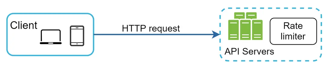
• Server-side implementation. Figure 1 shows a rate limiter that is placed on the server-side.

Besides the client and server-side implementations, there is an alternative way. Instead of putting a rate limiter at the API servers, we create a rate limiter middleware, which throttles requests to your APIs as shown in Figure 2.

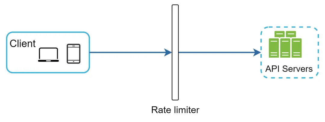
Figure 2
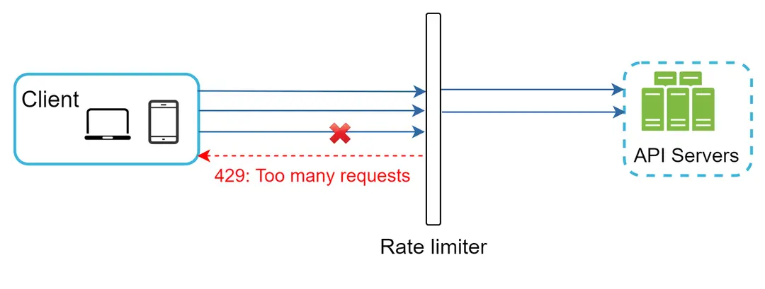
Let us use an example in Figure 3 to illustrate how rate limiting works in this design. Assume our API allows 2 requests per second, and a client sends 3 requests to the server within a second. The first two requests are routed to API servers. However, the rate limiter middleware throttles the third request and returns a HTTP status code 429. The HTTP 429 response status code indicates a user has sent too many requests.

Cloud microservices [4] have become widely popular and rate limiting is usually implemented within a component called API gateway.
Identify the rate limiting algorithm that fits your business needs. When you implement everything on the server-side, you have full control of the algorithm. However, your choice might be limited if you use a third-party gateway.
• If you have already used microservice architecture and included an API gateway in the design to perform authentication, IP whitelisting, etc., you may add a rate limiter to the API gateway.
Rate limiting can be implemented using different algorithms
• Token bucket
• Leaking bucket
• Fixed window counter
• Sliding window log
• Sliding window counter
The token bucket algorithm work as follows:
• A token bucket is a container that has pre-defined capacity. Tokens are put in the bucket at preset rates periodically. Once the bucket is full, no more tokens are added. As shown in Figure 4, the token bucket capacity is 4. The refiller puts 2 tokens into the bucket every second. Once the bucket is full, extra tokens will overflow.


Figure 4
• Each request consumes one token. When a request arrives, we check if there are enough tokens in the bucket. Figure 5 explains how it works.
• If there are enough tokens, we take one token out for each request, and the request goes through.
• If there are not enough tokens, the request is dropped.


Figure 5
Figure 6 illustrates how token consumption, refill, and rate limiting logic work. In this example, the token bucket size is 4, and the refill rate is 4 per 1 minute.


Figure 6
How many buckets do we need? This varies, and it depends on the rate-limiting rules. Here are a few examples.
• It is usually necessary to have different buckets for different API endpoints. For instance, if a user is allowed to make 1 post per second, add 150 friends per day, and like 5 posts per second, 3 buckets are required for each user.
• If we need to throttle requests based on IP addresses, each IP address requires a bucket.
• If the system allows a maximum of 10,000 requests per second, it makes sense to have a global bucket shared by all requests.
Pros:
• The algorithm is easy to implement.
• Memory efficient.
• Token bucket allows a burst of traffic for short periods. A request can go through as long as there are tokens left.
Cons:
• Two parameters in the algorithm are bucket size and token refill rate. However, it might be challenging to tune them properly.
The leaking bucket algorithm is similar to the token bucket except that requests are processed at a fixed rate. It is usually implemented with a first-in-first-out (FIFO) queue. The algorithm works as follows:
• When a request arrives, the system checks if the queue is full. If it is not full, the request is added to the queue.
• Otherwise, the request is dropped.
• Requests are pulled from the queue and processed at regular intervals.
Figure 7 explains how the algorithm works.


Leaking bucket algorithm takes the following two parameters:
• Bucket size: it is equal to the queue size. The queue holds the requests to be processed at a fixed rate.
• Outflow rate: it defines how many requests can be processed at a fixed rate, usually in seconds.
Pros:
• Memory efficient given the limited queue size.
• Requests are processed at a fixed rate therefore it is suitable for use cases that a stable outflow rate is needed.
Cons:
• A burst of traffic fills up the queue with old requests, and if they are not processed in time, recent requests will be rate limited.
• There are two parameters in the algorithm. It might not be easy to tune them properly.
Fixed window counter algorithm works as follows:
• The algorithm divides the timeline into fix-sized time windows and assign a counter for each window.
• Each request increments the counter by one.
• Once the counter reaches the pre-defined threshold, new requests are dropped until a new time window starts.
A major problem with this algorithm is that a burst of traffic at the edges of time windows could cause more requests than allowed quota to go through. Consider the following case:


Figure 9
In Figure 9, the system allows a maximum of 5 requests per minute, and the available quota resets at the human-friendly round minute. As seen, there are five requests between 2:00:00 and 2:01:00 and five more requests between 2:01:00 and 2:02:00. For the one-minute window between 2:00:30 and 2:01:30, 10 requests go through. That is twice as many as allowed requests.
Pros:
• Memory efficient.
• Easy to understand.
• Resetting available quota at the end of a unit time window fits certain use cases.
Cons:
• Spike in traffic at the edges of a window could cause more requests than the allowed quota to go through.
We explain the algorithm with an example as revealed in Figure 10.


Figure 10
In this example, the rate limiter allows 2 requests per minute. Usually, Linux timestamps are stored in the log. However, human-readable representation of time is used in our example for better readability.
• The log is empty when a new request arrives at 1:00:01. Thus, the request is allowed.
• A new request arrives at 1:00:30, the timestamp 1:00:30 is inserted into the log. After the insertion, the log size is 2, not larger than the allowed count. Thus, the request is allowed.
• A new request arrives at 1:00:50, and the timestamp is inserted into the log. After the insertion, the log size is 3, larger than the allowed size 2. Therefore, this request is rejected even though the timestamp remains in the log.
• A new request arrives at 1:01:40. Requests in the range [1:00:40,1:01:40) are within the latest time frame, but requests sent before 1:00:40 are outdated. Two outdated timestamps, 1:00:01 and 1:00:30, are removed from the log. After the remove operation, the log size becomes 2; therefore, the request is accepted.
Note: Sliding window log algorithm
Pros:
• Rate limiting implemented by this algorithm is very accurate. In any rolling window, requests will not exceed the rate limit.
Cons:
• The algorithm consumes a lot of memory because even if a request is rejected, its timestamp might still be stored in memory.
Figure 11 illustrates how this algorithm works.


Figure 11
Assume the rate limiter allows a maximum of 7 requests per minute, and there are 5 requests in the previous minute and 3 in the current minute. For a new request that arrives at a 30% position in the current minute, the number of requests in the rolling window is calculated using the following formula:
• Requests in current window + requests in the previous window ***** overlap percentage of the rolling window and previous window
• Using this formula, we get 3 + 5 * 0.7% = 6.5 request. Depending on the use case, the number can either be rounded up or down. In our example, it is rounded down to 6.
Since the rate limiter allows a maximum of 7 requests per minute, the current request can go through. However, the limit will be reached after receiving one more request.
Note: Sliding window counter algo
Pros
• It smooths out spikes in traffic because the rate is based on the average rate of the previous window.
• Memory efficient.
Cons
• It only works for not-so-strict look back window. It is an approximation of the actual rate because it assumes requests in the previous window are evenly distributed. However, this problem may not be as bad as it seems. According to experiments done by Cloudflare [10], only 0.003% of requests are wrongly allowed or rate limited among 400 million requests.
Where shall we store counters? Using the database is not a good idea due to slowness of disk access. In-memory cache is chosen because it is fast and supports time-based expiration strategy. For instance, Redis [11] is a popular option to implement rate limiting. It is an in-memory store that offers two commands: INCR and EXPIRE.
• INCR: It increases the stored counter by 1.
• EXPIRE: It sets a timeout for the counter. If the timeout expires, the counter is automatically deleted.
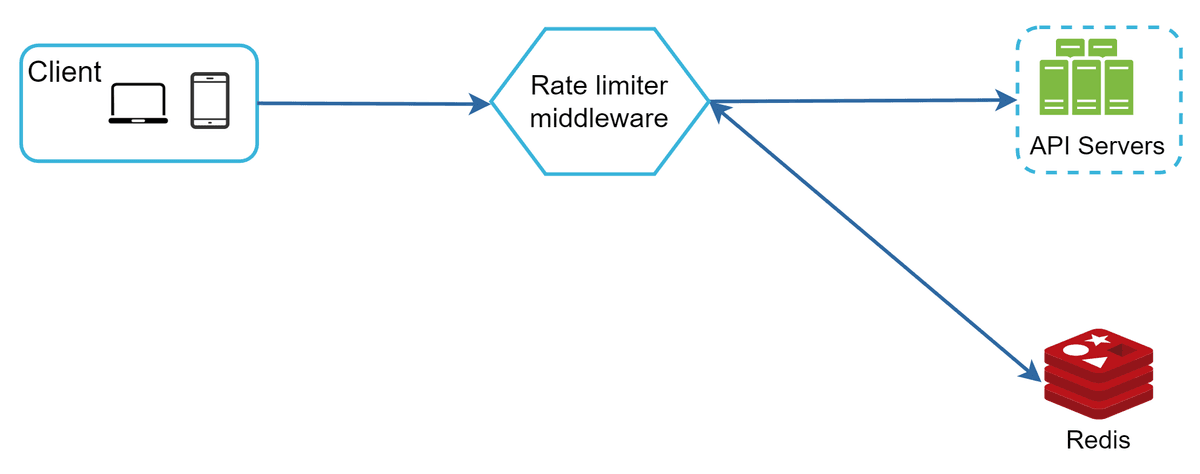
Figure 12 shows the high-level architecture for rate limiting, and this works as follows:

In case a request is rate limited, APIs return a HTTP response code 429 (too many requests) to the client. Depending on the use cases, we may enqueue the rate-limited requests to be processed later. For example, if some orders are rate limited due to system overload, we may keep those orders to be processed later.
The rate limiter returns the following HTTP headers to clients:
X-Ratelimit-Remaining: The remaining number of allowed requests within the window.

X-Ratelimit-Limit: It indicates how many calls the client can make per time window.

X-Ratelimit-Retry-After: The number of seconds to wait until you can make a request again without being throttled.
When a user has sent too many requests, a 429 too many requests error and X-Ratelimit-Retry-After header are returned to the client.
The rate limiter returns the following HTTP headers to clients:
X-Ratelimit-Remaining: The remaining number of allowed requests within the window.
X-Ratelimit-Limit: It indicates how many calls the client can make per time window.
X-Ratelimit-Retry-After: The number of seconds to wait until you can make a request again without being throttled.
When a user has sent too many requests, a 429 too many requests error and X-Ratelimit-Retry-After header are returned to the client.
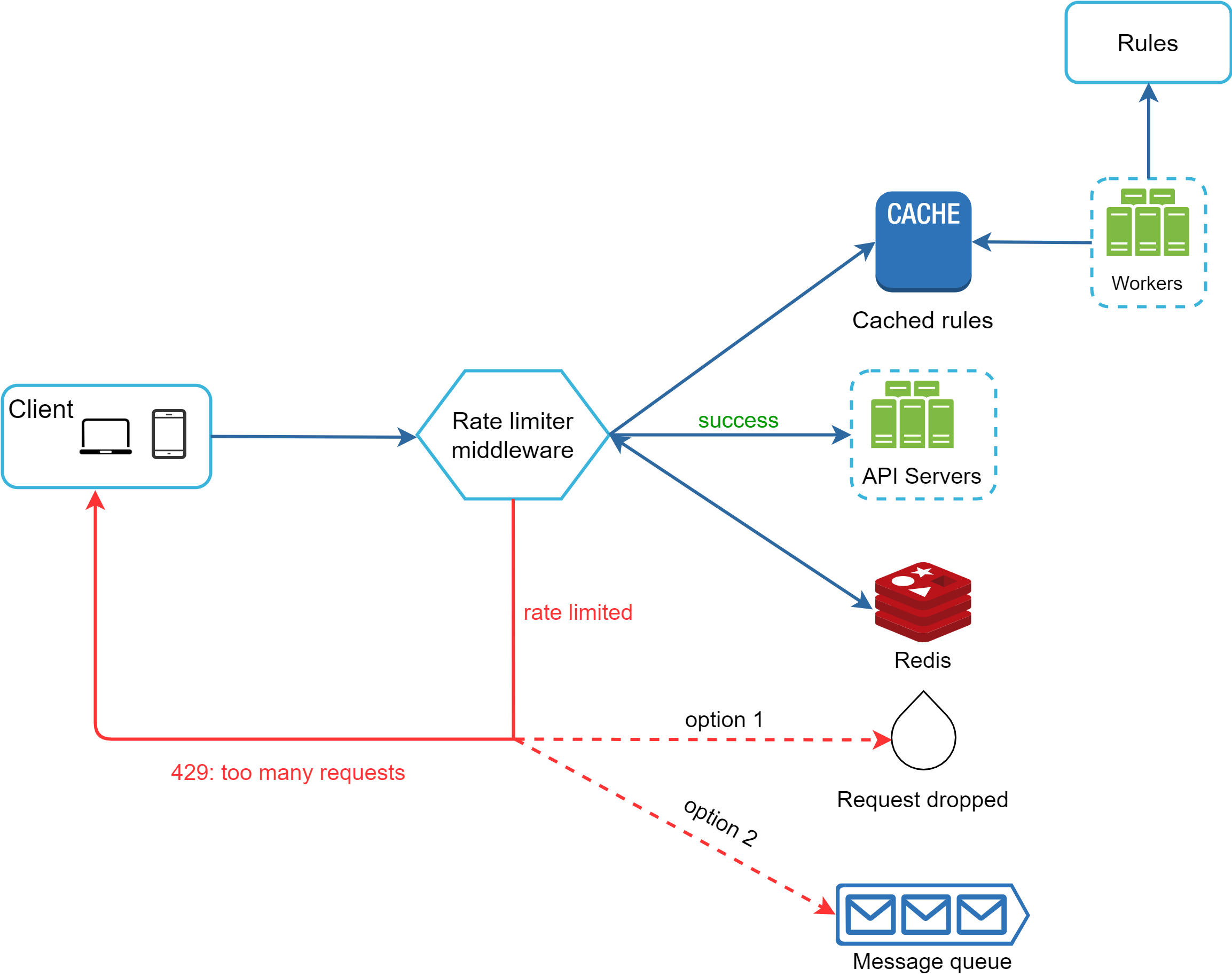
Figure 13
• Rules are stored on the disk. Workers frequently pull rules from the disk and store them in the cache.
• When a client sends a request to the server, the request is sent to the rate limiter middleware first.
• Rate limiter middleware loads rules from the cache. It fetches counters and last request timestamp from Redis cache. Based on the response, the rate limiter decides:
• if the request is not rate limited, it is forwarded to API servers.
• if the request is rate limited, the rate limiter returns 429 too many requests error to the client. In the meantime, the request is either dropped or forwarded to the queue.
Building a rate limiter that works in a single server environment is not difficult. However, scaling the system to support multiple servers and concurrent threads is a different story. There are two challenges:
• Race condition
• Synchronization issue
Race conditions can happen in a highly concurrent environment as shown in Figure 14.


Figure 14
Assume the counter value in Redis is 3. If two requests concurrently read the counter value before either of them writes the value back, each will increment the counter by one and write it back without checking the other thread. Both requests (threads) believe they have the correct counter value 4. However, the correct counter value should be 5.
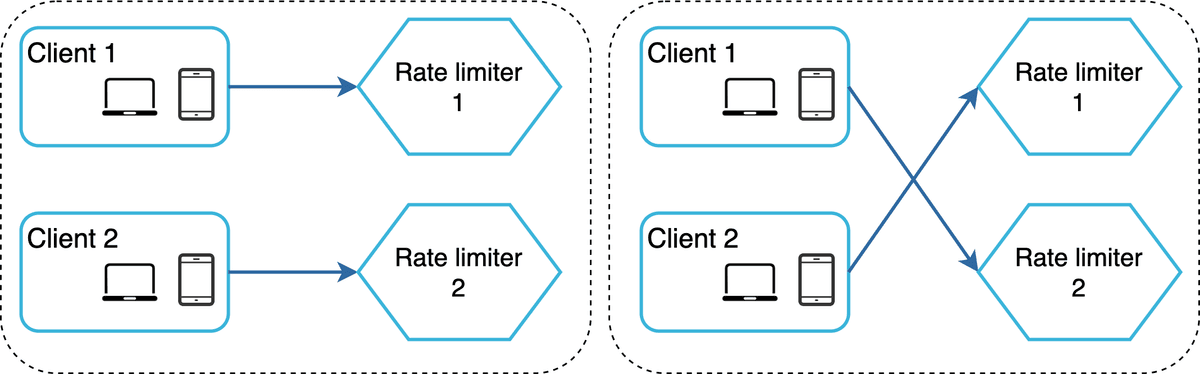
o support millions of users, one rate limiter server might not be enough to handle the traffic. When multiple rate limiter servers are used, synchronization is required. For example, on the left side of Figure 15, client 1 sends requests to rate limiter 1, and client 2 sends requests to rate limiter 2. As the web tier is stateless, clients can send requests to a different rate limiter as shown on the right side of Figure 15. If no synchronization happens, rate limiter 1 does not contain any data about client 2. Thus, the rate limiter cannot work properly.

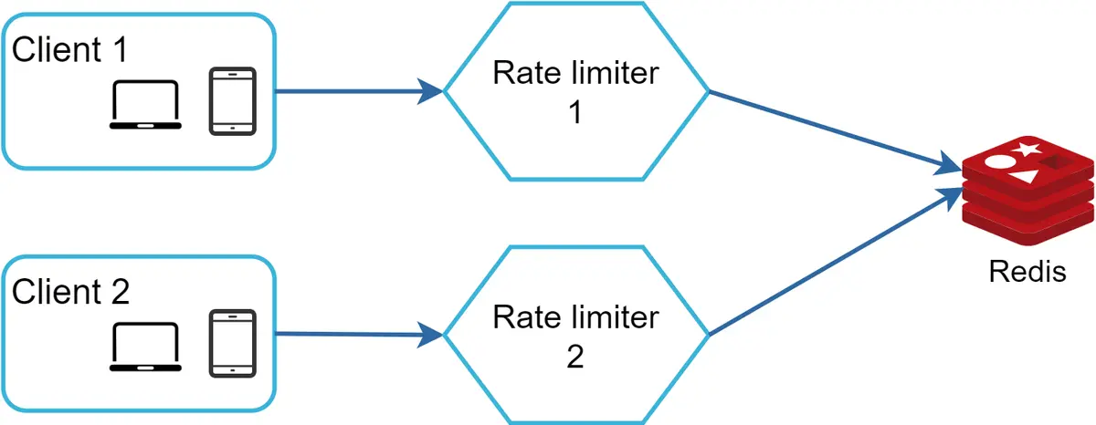
One possible solution is to use sticky sessions that allow a client to send traffic to the same rate limiter. This solution is not advisable because it is neither scalable nor flexible. A better approach is to use centralized data stores like Redis. The design is shown in Figure 16.

Rate limiting at different levels. In this chapter, we only talked about rate limiting at the application level (HTTP: layer 7). It is possible to apply rate limiting at other layers. For example, you can apply rate limiting by IP addresses using Iptables [15] (IP: layer 3). Note: The Open Systems Interconnection model (OSI model) has 7 layers [16]: Layer 1: Physical layer, Layer 2: Data link layer, Layer 3: Network layer, Layer 4: Transport layer, Layer 5: Session layer, Layer 6: Presentation layer, Layer 7: Application layer.